Machine Learning Model Selection with Metaflow

• AICamp recipe Github gist
• fwhigh/metaflow-helper Github project
• AICamp talk on YouTube

Overview

I worked with the Metaflow creators at Netflix from the time they built their first proofs of concept. About six months later I built my first flows as one of the earliest adopters. I had been rolling my own Flask API services to serve machine learning model predictions but Metaflow provided a much more accessible, lower complexity path to keep the models and services up to date.

I also had the privilege of working next to a lot of other talented developers who built some of their own spectacular ML based applications with Metaflow over the following years. Now that I’ve left Netflix I look forward to continuing to use it and helping others get the most out of it.

What is Metaflow? It’s a framework that lets you write data pipelines in pure Python, and it’s particularly suited to scaling up machine learning applications. Pipelines are specified as multiple steps in a flow, and steps can consist of potentially many tasks executed in parallel in their own isolated containers in the cloud. Tasks are stateless and reproducible. Metaflow persists objects and data in a data store like S3 for easy retrieval, inspection, and further processing by downstream systems. Read more at https://metaflow.org/.

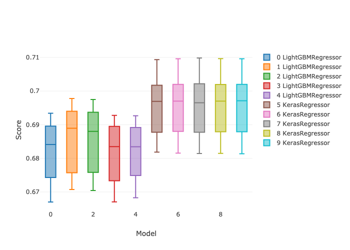
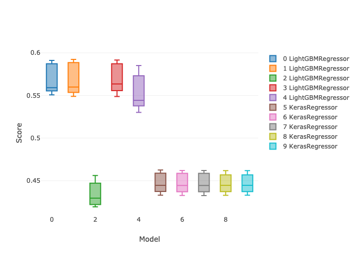
In this post I’ll demonstrate one of the ways I like to use it: doing repeatable machine learning model selection at scale. (This post does not address the ML model reproducibility crisis. Repeatable here means easily re-runnable.) I’ll compare 5 different hyperparameter settings for each of LightGBM and Keras regressors, with 5 fold cross validation and early stopping, for a total of 50 parallel model candidates. All of these instances are executed in parallel. The following box plots show the min and max and the 25th, 50th (median), and 75th percentiles of r-squared score from a mock regression data set.

Noisy regression, one category: any of the tested Keras architectures wins on out-of-sample r-squared score. The narrow single-hidden-layer Keras model happened to be best overall, with l1 factor 2.4e-7 and l2 factor 7.2e-6.

Noisy regression, two categories: LightGBM with depth 3 interactions and learning rate 0.03 wins on out-of-sample r-squared score. The LightGBM model with depth 1 performed the worst.

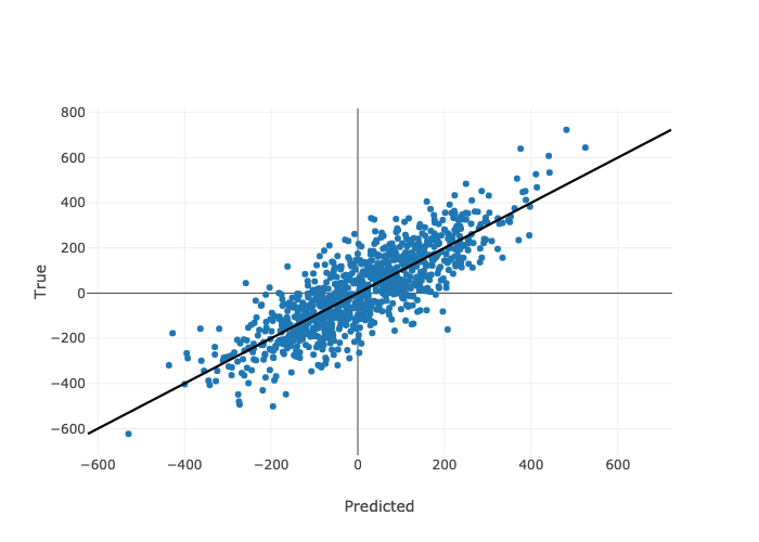
Predictions from the best model settings on the held out test set look like this for the noisy one-category data set.

Predicted versus true for the noisy regression, one category.

For just 2 models each on a hyperparameter grid of size 10 to 100, and using 5 fold cross validation, cardinality can reach between of order 100 to 1000 jobs. It’s easy to imagine making that even bigger with more models or hyperparameter combinations. Running Metaflow in the cloud (e.g. AWS) lets you execute each one of them concurrently in isolated containers. I’ve seen the cardinality blow up to of order 10,000 or more and things still work just fine, as long as you’ve got the time, your settings are reasonable, and your account with your cloud provider is big enough. With the

The code is available at https://github.com/fwhigh/metaflow-helper. The examples in this article are reproducible from the commit tagged v0.0.1. You can also install the tagged package from PyPI with pip install metaflow-helper==0.0.1. Comments, issues, and pull requests are welcome.

This post is not meant to conclude whether LightGBM is better than Keras or vice versa – I chose them for illustration purposes only. What model to choose, and which will win a tournament, are application-dependent. And that’s sort of the point! This procedure outlines how you would productionalize model tournaments that you can run on many different data sets, and repeat the tournament over time as well.

Quickstart

You can run the model selection tournament immediately like this. Install a convenience package called metaflow-helper at the commit tagged v0.0.1.

Then run the Metaflow tournament job at a small scale just to test it out. This one needs a few more packages, including Metaflow itself, which metaflow-helper doesn’t currently require.

Results are printed to the screen, but they are also summarized in a local file results/<run-id>/summary.txt along with some plots. There are full scale model selection configurations available in there as well.

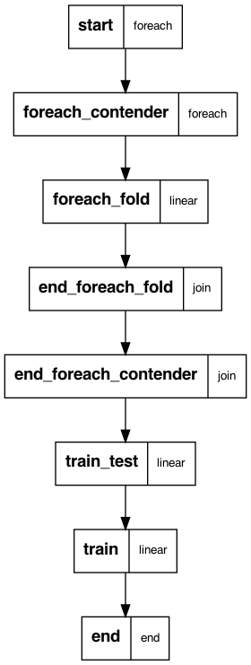
Following figure shows the flow you are running. The mock data is generated in the start step. The next step splits across all hyperparameter grid points for all contenders – 10 total for 2 models in the case of this example. Then there are 5 tasks for each cross validation fold, for a total of 50 tasks. Models are trained in these tasks directly. The next step joins the folds and summarizes the results by model and hyperparameter grid point. Then there’s a join over all models and grid points, whereupon a final model with a held out test set is trained and evaluated/ Finally a model on all of the data is trained. The end step produces summary data and figures.

Model selection flow.

Mocking A Data Set

The mock regression data is generated using Scikit-learn make_regression. Keyword parameter settings are controlled entirely in configuration files like randomized_config.py in an object called make_regression_init_kwargs. If you set n_categorical_features = 1 you’ll get a single data set with n_numeric_features continuous features, n_informative_numeric_features of which are “informative” to the target y, with noise given by noise, through the relationship y = beta * X + noise. beta are the coefficients, n_numeric_features - n_informative_numeric_features of which will be zero. You can add any other parameters make_regression accepts directly to make_regression_init_kwargs.

If you set n_categorical_features = 2 or more, you’ll get n_categorical_features independent regression sets concatenated together into a single data set. Each category corresponds to a totally independent set of coefficients. Which features are uninformative for each of the categories is entirely random. This is a silly construction but it allows for validation of the flow against at least one categorical variable.

Specifying Contenders

All ML model contenders, including their hyperparameter grids, are also specified in randomized_config.py using the contenders_spec object. Implement this spec object like you would any hyperparameter grid that you would pass to Scikit-learn GridSearchCV or RandomizedSearchCV, or equivalently ParameterGrid or ParameterSampler. Randomized search is automaticallly used if the '__n_iter' key is present in the contender spec, otherwise the flow will fall back to grid search.

Here’s an illustration of tuning two models. The LightGBM model is being tuned over 5 random max_depth and learning_rate settings. The Keras model is being tuned over 5 different combinations of layer architectures and regularizers. The layer architectures are

• no hidden layers,
• one hidden layer of size 15,
• two hidden layers each of size 15, and
• one wide hidden layer of size 225. The regularizers are l1 and l2 factors, log-uniformly sampled and applied globally to all biases, kernels, and activations. This specific example may well be a naive search, but the main purpose right now is to demonstrate what is possible. The spec can be extended arbitrarily for real-world applications.

The model is specified in a reserved key, '__model'. The value of '__model' is a fully qualified Python object path string. In this case I’m using metaflow-helper convenience objects I’m calling model helpers, which reimplement init, fit, and predict with a small number of required keyword arguments.

Anything prepended with '__init_kwargs__model' gets passed to the model initializers and '__fit_kwargs__model' keys get passed to the fitters. I’m wrapping the model in a Scikit-learn Pipeline with step-name 'model'.

I implemented two model wrappers, a LightGBM regressor and a Keras regressor. Sources for these are in metaflow_helper/models. They’re straightforward, and you can implement additional ones for any other algo.

Further Ideas and Extensions

There are a number of ways to extend this idea.

Idea 1: It was interesting to do model selection on a continuous target variable, but it’s possible to do the same type of optimization for a classification task using Scikit-learn make_classification and make_multilabel_classification to mock data.

Idea 2: You can add more model handlers for ever larger model selection searches.

Idea 3: It’d be especially interesting to try to use all models in the grid in an ensemble, which is definitely also possible with Metaflow by joining each model from parallel grid tasks and applying another model of models.

Idea 4: I do wish I could simply access each task in Scikit-learn’s cross-validation search (e.g. GridSearchCV) tasks and distribute those directly into Metaflow steps. Then I could recycle all of its Pipeline and CV search machinery and patterns, which I like. I poked around the Scikit-learn source code just a bit but it didn’t seem straightforward to implement things this way. I had to break some Scikit-learn patterns to make things work but it wasn’t too painful.

I’m interested in any other ideas you might have. Enjoy!