
The Streaming Distributed Bootstrap
The bootstrap (Efron 1979) is an incredibly practical method to estimate uncertainty from finite sampling on almost any quantity of interest. If, say, you’re training a model using just 30 training examples, you’ll likely want to know how uncertain your goodness-of-fit metric is. Is your AUC statistically consistent with 0.5? That’d be key to know, and you could estimate it with the bootstrap.
The standard bootstrap, however, does not scale well to big data, and for unbounded data streams it’s in fact not well defined. The standard bootstrap assumes you have all your data locally available, it’s static, it fits into primary memory, and it’s easy to compute your metric of interest (AUC in the above example).
There has been lots of exciting new research around scaling the bootstrap to unbounded and distributed data. The Bag of Little Bootstraps paper distributes the bootstrap, but issues a standard “static” bootstrap on each thread, so it doesn’t solve the unbounded data problem. The Vowpal Wabbit paper solves the unbounded data problem, but on a single thread. A Google paper puts together a bootstrap that is both streaming and distributed.
The streaming distributed bootstrap is a really fun solution, and I’ve mocked up a Python package to test it out. In this article, I’m going to assume you’re already a fairly technical person who understands why you’d want to estimate uncertainty on a big data application.
At the end of this post I’ll set loose a streaming bootstrap on the Twitter firehose, computing the mean tweet rate on top trending terms at the time I ran it, with streaming one-sigma error bands.
I’ll be using the following R libraries and global settings for the R snippets.
Refresher: the standard bootstrap
Let’s start with a fake data set of $N=30$ points, and let’s say the data is drawn from a random uniform distribution.
Here’s what it looks like.
    index count      value
 1:     1     1 0.23666352
 2:     2     1 0.17972139
 3:     3     1 0.04451190
 4:     4     1 0.94861152
 5:     5     1 0.97012678
 6:     6     1 0.11215551
 7:     7     1 0.81616358
 8:     8     1 0.71385778
 9:     9     1 0.54395965
10:    10     1 0.03084962
11:    11     1 0.58808657
12:    12     1 0.03196848
13:    13     1 0.78770594
14:    14     1 0.57319726
15:    15     1 0.23914206
16:    16     1 0.45210949
17:    17     1 0.74648136
18:    18     1 0.76919459
19:    19     1 0.50524423
20:    20     1 0.68976405
21:    21     1 0.88024924
22:    22     1 0.52815155
23:    23     1 0.03672133
24:    24     1 0.16118379
25:    25     1 0.23268336
26:    26     1 0.51450148
27:    27     1 0.18569415
28:    28     1 0.54663857
29:    29     1 0.89967953
30:    30     1 0.34810339
    index count      value
The index identifies the data point, the count is simply the number of times that data point appears, and the value is “the data.” The mean of the data is 0.48 and the standard error on the mean is 0.05.
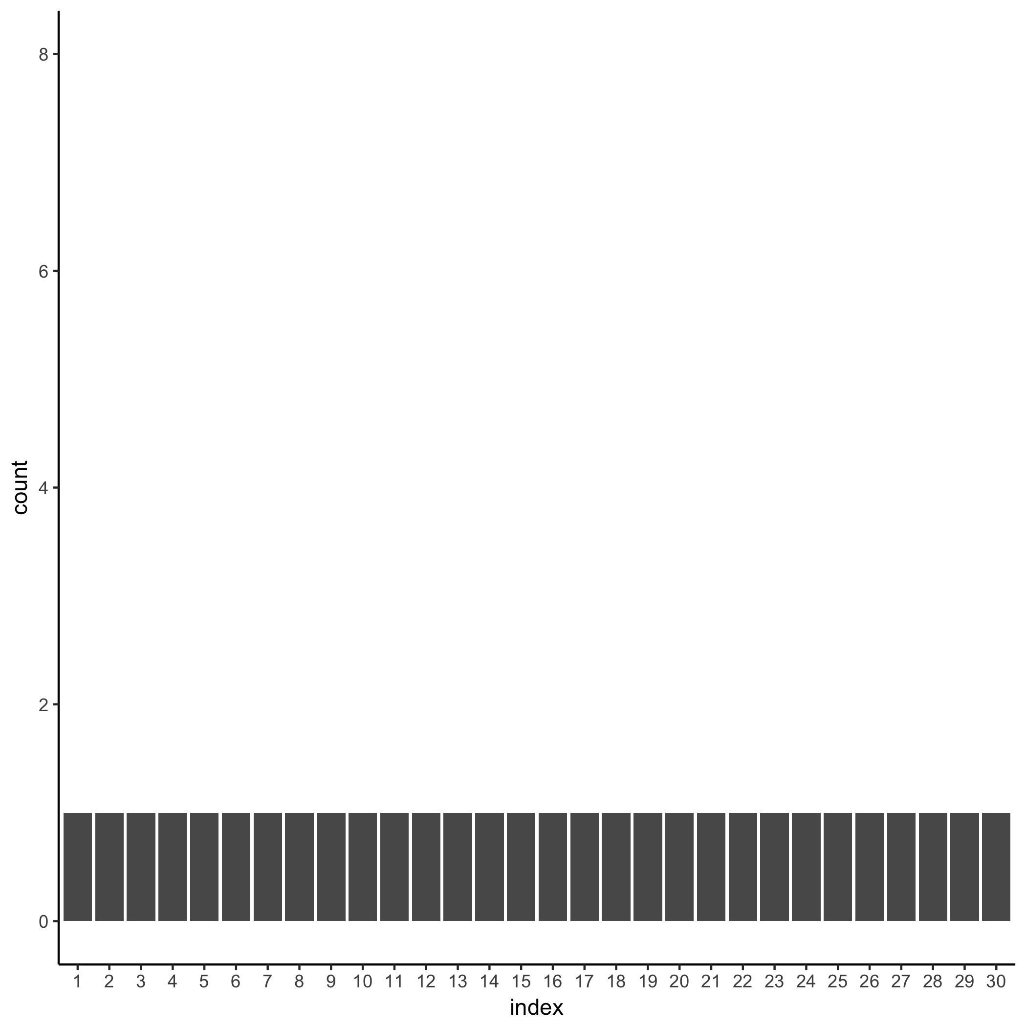
I’m going to start by histogramming the counts of each index. This is a trivial histogram: there’s just one of everything.
Now the bootstrap procedure is
- resample the $N$ data points $N$ times with replacement,
- compute your quantity of interest on the resampled data exactly as if it was the original data, and
- repeat hundreds or thousands of times.
The resulting distribution of the quantity of interest is an empirical estimate of the sampling distribution of that quantity. This means the mean of the distro is an estimate of the quantity of interest itself, and the standard deviation is an estimate of the standard error of that quantity. That last point is tricky and worth memorizing to impress your statistics friends at parties. (Just kidding, statisticians don’t go to parties!)
Here’s an implementation of the bootstrap for this data set. The quantity of interest in this example is the mean of the data.
My session gives me
compare bootstrap mean 0.477468987332949 to sample quantity of interest 0.477104055796129
compare bootstrap standard deviation 0.0547528263387387 to the sample standard error of the quantity of interest 0.0555938381440978
So both the bootstrap mean and the data mean are consistent with the population mean of 0.5 within one standard error of the mean, and the analytical estimator of the standard error is consistent with the bootstrap standard deviation. All is good.
Thinking more deeply about the resampling
Now it gets interesting. It turns out that step #1 in the bootstrap procedure can be thought of as rolling an unbiased $N$ sided dice $N$ times, and counting the number of times each face (index) comes up. This is a result from elementary statistics: the counts of each face is distributed as
\begin{equation} \mathrm{Multinomial}(N,\pmb{p}=(1/N,1/N,\dots,1/N)), \end{equation}
where $\pmb{p}$ is a vector of $N$ probabilities. I’m going to simulate one single bootstrap iteration like this:
Here’s a histogram of the number of times each data point comes up in this iteration:
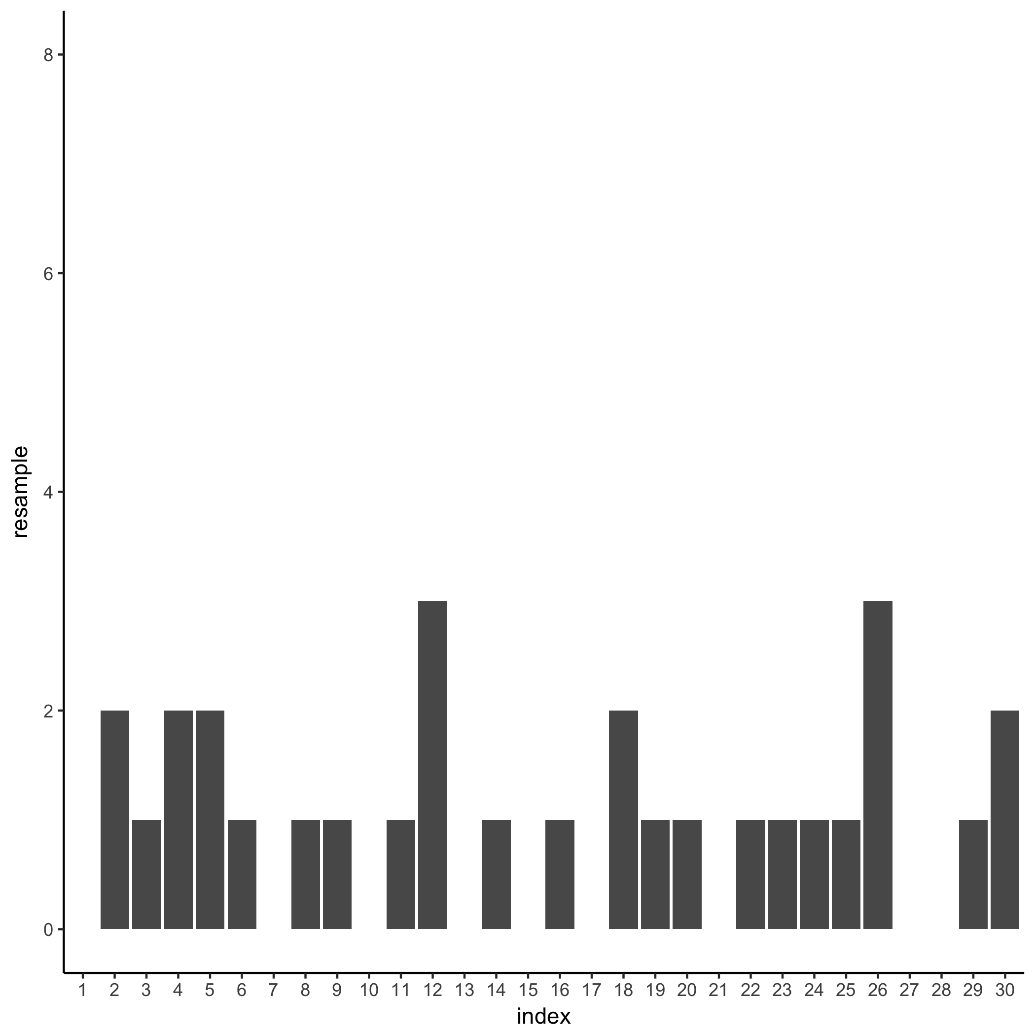
A bunch of points are resampled zero times, the 12th and 26th data points are resampled 3 times, and everything else is in between. I already know the resample counts are Multinomially distributed, but here’s a slightly different question: over the course of a full bootstrap simulation, what’s the distribution of the sample rate of just the first data point?
This time the answer comes from thinking about coin tosses. In one single draw in one bootstrap iteration, the chances the first data point will be drawn is $1/N$. This is like flipping a coin that is biased as $p=1/N$. $N$ draws with replacement in one bootstrap iteration are like flipping that coin $N$ times, so the number of times the first data point comes up in one bootstrap iteration is distributed as $\mathrm{Binomial}(N,1/N)$.
You can simulate this effect for 10000 bootstrap iterations in R by picking out the first row of 10000 Multinomial random number draws. I’m going to do this, then count the number of time each draw frequency per bootstrap iteration occurs, then compare the the Binomial random draw.
Let’s take a look:
   frequency count    binomial
1:         0  3630 3678.610464
2:         1  3698 3678.978362
3:         2  1907 1839.489181
4:         3   607  613.101738
5:         4   135  153.244776
6:         5    17   30.639760
7:         6     6    5.104584
Math works.
The leap to big data: the Poisson trick
So far I’ve been dealing with small data, at $N = 30$. With big data $N$ is either very large or, more often, unknown. Let’s think about what happens when $N$ gets huge.
As $N$ grows the probability $p = 1/N$ of drawing the first data point is getting tiny, but the number of draws in a single bootstrap iteration is getting huge with $N$. It turns out this process converges, and the number of times you’d expect to see the first data point is Poisson distributed with mean 1. That is to say,
\begin{equation} \mathrm{Binomial}(N,1/N) \xrightarrow{N\to\infty} \mathrm{Poisson}(1). \end{equation}
The resampling procedure is independent of $N$! This was purely luck, and it means I don’t need to know the size of the full data set to bootstrap uncertainty estimates, and in fact if $N$ is large enough the bootstrapping procedure is nearly exact.
Let’s take a look.
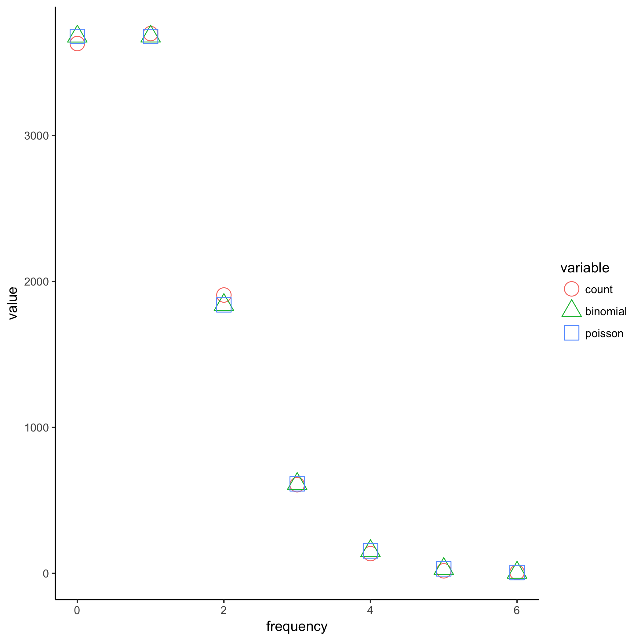
The agreement between the Binomial and Poisson distributions is already extremely good at just $N=30$, and it only gets better with large $N$. Because the Poisson distribution is independent of the parameter $N$, I can turn the entire bootstrap process sideways: I’ll run 10000 bootstraps on each data point as it arrives in the stream, without regard to what will stream in later, as long as I can define an online update rule for the metric of interest.
A streaming bootstrap of the mean
The mean as the quantity of interest is a useful example because it has a simple update rule. Pseudocode of the online weighted mean update rule is as follows.
Algorithm: WeightedMeanUpdate
Input: Current mean, theta0
       Aggregate weight of current mean, w0
       New data, X
       Weight of new data, W
Output: Updated mean, theta1
        Aggregate weight of updated mean, w1
theta1 = (w0*theta0 + W*X)/(w0 + W)
w1 = w0 + W
return (theta1,w1)
When W = 1, this reduces to an online unweighted mean update rule. For the very first data point, the mean and aggregate weight are set to 0.
Using the Poisson trick, the streaming serial bootstrap algorithm is:
Algorithm: StreamingSerialBootstrap
Input: Unbounded set of data-weight tuples {(X[1],w[1]),(X[2],w[2]),...}
       Number of bootstrap realizations, r
Output: Estimator value in each bootstrap realization, theta[k], k in {1,2,..,r}
// initialize
for each k in 1 to r do
  wInner[k] = 0
end
// data arrives from a stream
for each i in stream
  // do r bootstrap iteration
  // approximate resampling with replacement with the Poisson trick
  for k in 1 to r do
    weight = wInner[i]*PoissonRandom(1)
    (thetaInner[k],wInner[k]) = InnerOnlineUpdate(thetaInner[k],wInner[k],X[i],weight)
  end
end
The InnerOnlineUpdate must be set to WeightedMeanUpdate for the mean as the quantity of interest. thetaInner is an array representing a running estimate of the sample distribution of the mean at the $i$-th data point.
I’ve mocked this up in a Python package called sdbootstrap. First export the R data to file.
Then in the terminal,
The output is
- master update ID, which is the timestamp of the update,
- bootstrap iteration ID,
- quantity of interest,
- number of total resamples
Here are my top 10 lines:
1497630831.95 0 0.498431696583 35.0
1497630831.95 1 0.497802280908 32.0
1497630831.95 2 0.52108250027 34.0
1497630831.95 3 0.52590605129 34.0
1497630831.95 4 0.396820495147 26.0
1497630831.95 5 0.552172223237 32.0
1497630831.95 6 0.494006591897 29.0
1497630831.95 7 0.491453935547 27.0
1497630831.95 8 0.524614127751 31.0
1497630831.95 9 0.49028054256 25.0
The bootstrap mean (mean of column 3) is 0.4784 and the bootstrap standard error (standard deviation of column 3) is 0.0551, both close to the regular bootstrap values 0.4775 and 0.0548. So this seems to work fine even on just 30 data points.
Distributing it
Here’s a picture of what I’m about to construct.

I’ll do it by way of example. Let’s generate $N = 10000$ data points uniformly distributed between 0 and 1 with awk’s random number generator.
My top 10 entries are
0.237788 1
0.291066 1
0.845814 1
0.152208 1
0.585537 1
0.193475 1
0.810623 1
0.173531 1
0.484983 1
0.151863 1
A traditional bootstrap at 10000 iterations in R gives me
compare bootstrap mean 0.498704013190406 to sample quantity of interest 0.49865821011823
compare bootstrap standard deviation 0.00287165409456161 to the sample standard error of the quantity of interest 0.00288191093375261
The Bag of Little Bootstrap authors pointed out that you can multithread the bootstrap by doing a bunch of independent bootstraps and collecting the results. Their approach is to over-resample the data and summarize immediately in each thread, then collect, but I want to maintain the full bootstrap distribution so I’ll do it a little differently. And importantly, I’ll do it for unbounded data: each thread will do the job of the streaming bootstrap in the previous section, and it won’t know how big the full data set is.
This algo reuses the above StreamingSerialBootstrap in what I’m calling the inner bootstrap, and also implements an outer bootstrap procedure that collects each bootstrap iteration’s current state and does a aggregation to produce the a master bootstrap distribution.
Algorithm: StreamingDistributedBootstrap
Input: Unbounded set of data-weight tuples {(X[1],w[1]),(X[2],w[2]),...}
       Number of bootstrap realizations, r
       Number of nodes, s
Output: Estimator value in each bootstrap realization, theta[k], k in {1,2,..,r}
// initialize
for each k in 1 to r do
  wOuter[k] = 0
  for each j in 1 to s do
    wInner[j,k] = 0
  end
end
// data arrives from a stream
for each i in stream
  Assign tuple (X[i],w[i]) to node j in {1,2,...,s}
  // inner bootstrap
  // do r bootstrap iterations
  // approximate resampling with replacement with the Poisson trick
  for k in 1 to r do
    weight = wInner[i]*PoissonRandom(1)
    (thetaInner[j,k],wInner[j,k]) = InnerOnlineUpdate(thetaInner[j,k],wInner[j,k],X[i],weight)
  end
  if UpdateMaster() do
    (thetaMaster[k],wMaster[k]) = OuterOnlineUpdate(thetaMaster[k],wMaster[k],thetaInner[j,k],wInner[j,k])
    // flush the inner bootstrap distros
    thetaInner[j,k] = 0
    wInner[j,k] = 0
  end
end
For the mean, set both InnerOnlineUpdate and OuterOnlineUpdate to WeightedMeanUpdate. thetaMaster is a running estimate of the sample mean at the $i$-th data point.
Here it is with the Python package. I’m going distribute the data over 6 threads using the lovely Gnu parallel package (brew install parallel).
My top 10 output lines are
1497631385.97 5988 0.500353215188 9843.0
1497631385.97 5989 0.495968983126 10111.0
1497631385.97 5982 0.504122756197 9995.0
1497631385.97 5983 0.497282486683 10121.0
1497631385.97 5980 0.500647175678 10013.0
1497631385.97 5981 0.493803255786 9907.0
1497631385.97 5986 0.497372163828 10076.0
1497631385.97 5987 0.500258192842 9963.0
1497631385.97 5984 0.495168146999 10054.0
1497631385.97 5985 0.499804540368 10074.0
I’m getting a streaming distributed bootstrap mean of 0.49871 and a streaming distributed bootstrap standard deviation of 0.0028622 (compare to standard bootstrap values 0.49866 and 0.0028821, and to the direct data estimates 0.49866 and 0.0028819).
This example and a lot of thinking convinces me that the algorithm is right and my implementation is right. It is certainly not a complete or rigorous proof, I leave that to others.
Testing it on the Twitter firehose
Just for fun, let’s set this loose on some Twitter search terms. This simplest average quantity I could think of was the mean time between tweets for different terms. Let’s call this inter-tweet time.
I’m accessing the firehose via the t command line utility. The top trending term at the time of writing is “Whole Foods”. Here’s what some of the tweet data look like.
ID,Posted at,Screen name,Text
875734500466081796,2017-06-16 15:19:09 +0000,RogueInformant,@ALT_uscis @amazon @WholeFoods How long until @WholeFoods offers its own credit card? 15% off you first 5 bundles o… https://t.co/fifTNCPlMs
875734502785548288,2017-06-16 15:19:10 +0000,Fronk83,RT @CNET: Grocery a-go-go:  #Amazon to buy #WholeFoods for $13.7 billion $AMZN https://t.co/zF72YYe2Fo https://t.co/3dURTz7Rup
875734510230491136,2017-06-16 15:19:12 +0000,ultramet,So does this mean that @WholeFoods employees will now be treated in the same crappy way Amazon employees are? Feel bad for them.
875734517562183680,2017-06-16 15:19:14 +0000,framhammer,"RT @JacobAWare: Amazon, based on your recent purchase of #WholeFoods, you might also like:
• South Park season 19 on blu-ray
• asparagus water"
875734520993120256,2017-06-16 15:19:14 +0000,osobsamantar,"@GuledKnowmad @JeffBezos @amazon @WholeFoods Not any kind of milk, organic almond milk"
875734524080119808,2017-06-16 15:19:15 +0000,ChrisArvay,"#Roc @Wegmans Your move!
@amazon buys @WholeFoods https://t.co/p2Nq1DXLal"
I’ll convert the date to a timestamp in seconds and subtract the timestamp of the previous line, skipping the first one line of course.
I’ll make use of a Gnu utility called stdbuf (brew install gstdbuf from Homebrew on my Mac) that lets me disable the buffering that the awk stage is apparently inspiring. With no buffering I can turn on the firehose and get real-time updates of the bootstrap distribution at every 10 tweets.
I’m disabling the inner bootstrap flush so that I can look at the cumulative effect of all data as a function of time. Normally I need to flush the inner bootstrap estimates upon updating the master outer bootstrap distribution.
And I’m not parallelizing the inner bootstraps per trending term because I have just one data stream each – so this is not a full blown demo but it’s still cool and suggestive.
I let it run for rew minutes. Plotting it up:
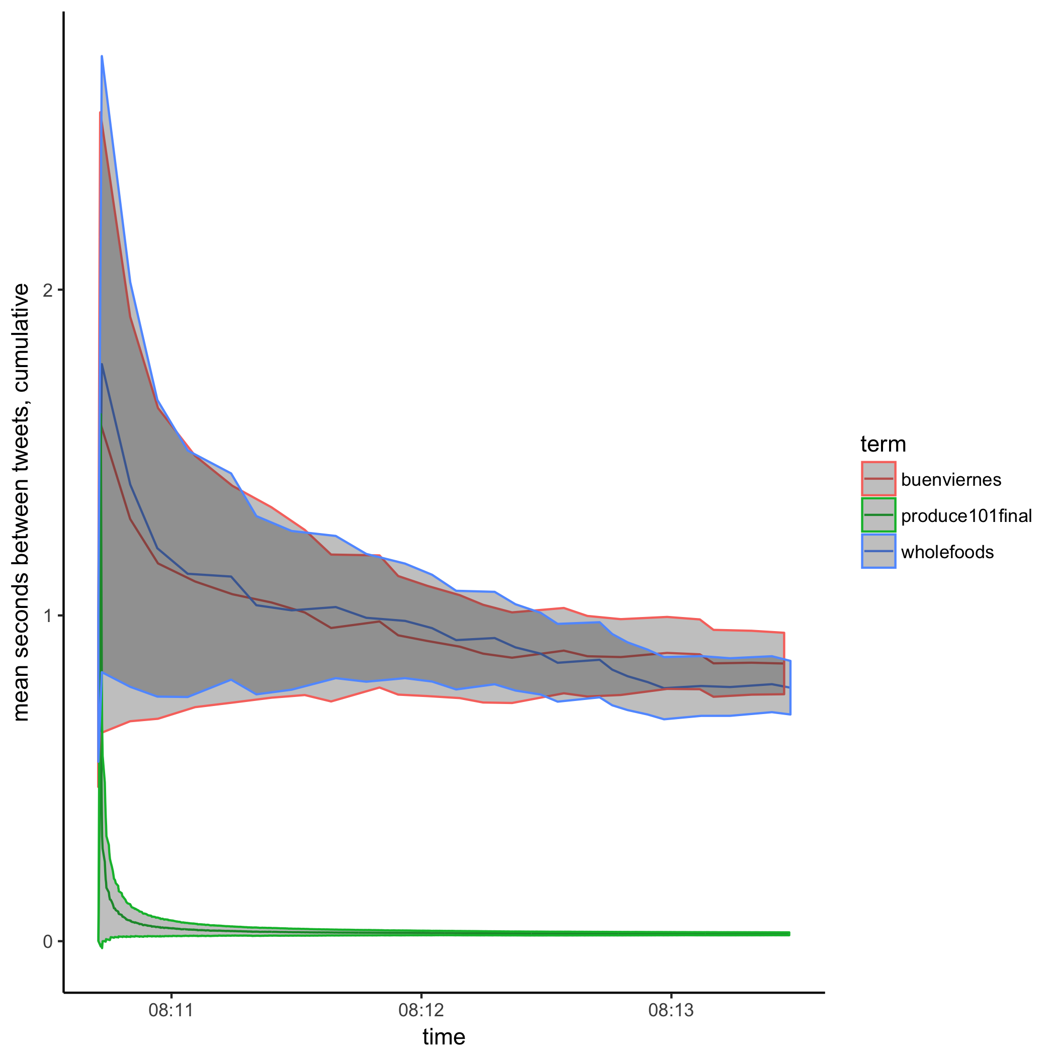
The top term is significantly more popular than the next two, which themselves are indistinguishible from one another over the period I accumulated data.
While I did not distribute each trending term’s bootstrap, I did already demo parallelizing the weighted mean bootstrap above so hopefully that’s enough to convince you that it’s possible over distributed Twitter streams.
Summary
I’ve sketched the train of logic that takes you from the standard bootstrap, to the streaming flavor, to the streaming-and-distributed flavor, and I did a cute Twitter firehose example. The purpose of this approach was not to prove anything rigorously but to make the concepts real and build deep intuition by actually doing it.
This is not the streaming version of the Bag of Little Bootstrap. The BLB (1) maintains over-resampled bootstrap distributions over each shard and (2) immediately summarizes the sharded bootstraps locally on their own threads, then (3) collects and aggregates the summaries themselves to create a more precise summary. What I’ve done here is maintain exact streaming bootstraps over each shard and collected the full bootstrap distribution in a downstream master thread, then summarized. For the weighted mean and many data points, the streaming distributed bootstrap is equivalent to a single standard bootstrap. This is true for any online update rule that can handle aggregated versions of the statistic of interest. In cases where the update rule cannot handle aggregate versions of the statistic, maybe you’d just do a weighted mean update to compute the master bootstrap distribution.
You can play many variations on this theme, as I’ve done a bit in this post, choosing any combination among
- online or batch
- distributed or single threaded
- master bootstrap distribution thread or immediate mean & standard-deviation summarization
I’ve toyed with more statistics, like quantiles and the exponentially weighted moving average (EWMA), both of which can be computed online. You can take a look at these updaters at https://github.com/fwhigh/sdbootstrap/tree/master/sdbootstrap/updater.
Comments